Library of machine learning
Models developed from scratch
Distinguish between cows, goats and sheep from the pixels of their images. Understanding models developed in Rust and explain their decisions.
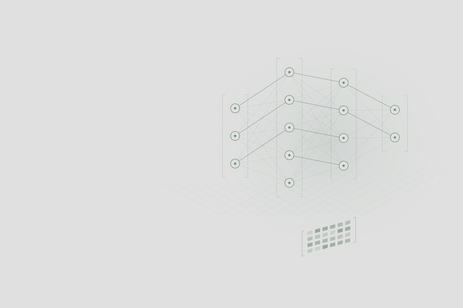
Three species, a progression in models
- 1. Prepare for what the model seesThe photo, its pixels, its label.
- 2. Understand the three modelsLinear: add. RBF: compare to centers. MLP: learning from transformations.
- 3. Examine their decisions2D borders, image experiments and confusions, then photo testing.
1 / 3 · From photos to models
Cow, goat or sheep: learn to distinguish the three
A photo arrives in the application. The goal is to choose between cow, goat and sheep based on its pixels. To understand what makes this recognition possible — and what resists it — the project is building a library of models from scratch in Rust, controlled from Python.
A concrete problem to understand the calculations
We will prepare the images, understand a linear combination, add local landmarks with the RBF, then layers learned with the MLP. Then, the experiments of each model will make it possible to link its decisions to its operation. At the end, you will be able to classify photos from the dataset.
Click in the image to read its three values
The cursor allows the same keyboard exploration. We read R, G, B, then the next pixel: 40 × 40 × 3 = 4,800 coordinates. Normalized values use the minimum and maximum of the entire photo.
1 / 3 · From photos to models
A goat becomes 4,800 numbers
We recognize a head, legs or a silhouette. The model receives only a 40 × 40 pixel image, with three values per pixel: red, green and blue. By reading the lines successively, we obtain a vector of 4,800 coordinates. The position of each value remains fixed.
Why impose the same format?
A model always expects the same number of inputs. Converting images to RGB prevents a photo in grayscale or with transparency from producing a different length. Min–max normalization of each image reduces its values to between 0 and 1. Resizing saves computation, but useful details, like fur texture, become difficult to distinguish.
Same input, one target to learn
Goat → [−1, +1, −1]
Sheep → [−1, −1, +1]
- 1. Learn about labeled imagesCorrections modify the weights; the photo does not change.
- 2. Freeze the modelThe rating prediction does not adjust any parameters.
- 3. Compare predicted class and expected classA photo gives only one answer, even if three scores are calculated.
1 / 3 · From photos to models
Show the photo, then correct the answer
Folders associate each image with a class. For a goat, the target is [−1, +1, −1], in the order cow, goat, sheep. The model calculates three scores; the index of the largest determines its answer. Learning involves adjusting the parameters to bring these scores closer to the target.
Why isn't one good answer enough?
A model can succeed in photos already used and fail in a new pose. It is therefore necessary to separate the training images from those for evaluation, and keep a photo and its augmented variants in the same group. We will distinguish the results announced in the report from the diagnostics recalculated on the backups.
One pixel contributes; he doesn't decide alone
goat score = tanh(z goat)
Contribution of this channel: 0.5 × 0.8 = 0.4. The other 4,799 values and the bias also participate.
Values that can be manipulated to understand the equation; this weight is not extracted from a prediction. Each class has its own weights.
2 / 3 · Understanding models
One weight per pixel value, three scores to decide between
The linear model assigns each RGB value a weight for each of the three classes. It multiplies the pixels by these weights, adds the contributions and adds a bias. A positive weight pushes the score up; a negative weight reduces it. The tanh output bounds the result between −1 and +1.
Why start with him?
We can follow his entire decision: 4,800 contributions and a bias per class, or 14,403 parameters. But it combines pixels directly, without learning any intermediate representation. In a two-coordinate view, the boundary between two classes is a straight line. In 4,800 dimensions, it is a hyperplane: adding pixels does not change the linear nature of the separation.
Correct the goat score of a simplified example
z = 0.4 · goat target = +1
- 1. Error: 1 − 0.4 = 0.6The affine output is too low for this class.
- 2. Δw = α × 0.8 × 0.6Correction: 0.048. The bias also receives α × 0.6.
- 3. New weight: 0.548The contribution of this pixel goes from 0.4 to 0.438.
Only one channel is represented to follow the calculation. In the image, the 4,800 weights are corrected, for each of the three outputs.
2 / 3 · Understanding models
An error indicates which direction to move the weights
Let's imagine a goat whose goat score is too low. Active pixels receive a correction which increases this score during a future presentation. The learning rate α regulates the amplitude of the change: too large, it can cause the parameters to oscillate; too small, learning progresses slowly.
What exactly this implementation does
The linear drive corrects the affine output z with w ← w + α × x × (target − z), without derivative of tanh. The prediction then applies tanh. This function is increasing: it preserves the order of the scores as long as rounding does not make them equal. A reduction in numerical error therefore does not, in itself, prove better classification.
One center, one response zone
Usual Gaussian: 0.88
Solid line: exp(−distance⁴ / γ²), Rust code formula. Dotted lines: exp(−γ × distance²). Here the position varies on an axis to make the distance visible; γ does not have the same interpretation in the two formulas.
Multiple centers produce multiple responses, combined by the output weights. The photos illustrate the problem in question; this curve explains a mechanism, without constituting an RBF trained on their pixels.
2 / 3 · Understanding models
Replace the single line with proximity zones
If several groups of images of the same species are far apart, a single linear separation may be insufficient. The RBF principle involves placing centers, measuring the distance to each, and then combining their local responses. For images, a center would be an average vector of pixels: not necessarily a real photo or a recognizable animal.
Why use K-means before linear output?
K-means alternates assignment to the closest center and movement of the center towards the average of its group. It builds benchmarks without using labels. The output weights then learn to combine these proximities to classify. The library provided, however, works with points (x, y): it does not have an operational image version.
Compare the scope of two local functions
Usual Gaussian: 0.88
Solid line: exp(−distance⁴ / γ²), Rust code formula. Dotted lines: exp(−γ × distance²). Here the position varies on an axis to make the distance visible; γ does not have the same interpretation in the two formulas.
2 / 3 · Understanding models
A center that is too local no longer recognizes its neighbours
A strong activation means that the entrance resembles the center according to the chosen distance. Very narrow zones isolate the examples; very large areas give close responses for different inputs. The number of centers and their range determine the fineness of the separation.
Why does the exact formula matter?
The usual principle uses exp(−γ × distance²). The Rust code provided further squares the distance and calculates exp(−distance⁴ / γ²): the transition therefore does not have exactly the same shape. The visual allows you to compare the two. The 2D workshop uses the usual Gaussian form; its results describe this educational adaptation.
4,800 values → 50 → 50 → 3 scores
Some neurons are drawn to keep the connections readable. Each connection corresponds to a learned weight; biases are not represented.
- Pixels: positions and colorsThe photo comes in without a description of "horn" or "wool".
- Hidden layers: learned combinationsActivations can combine contrasts. To assign a precise concept to them would require analyzing them.
- Output: cow, goat, sheepThe highest score chooses a class.
2 / 3 · Understanding models
Learn transformations instead of fixing distance
MLP retains the weighted sums of the linear model, but inserts hidden layers and tanh activation after each layer. The neurons no longer just compare the photo to centers: they learn combinations of pixels, then combinations of these responses.
Why are activations essential?
Two successive linear layers are reduced to a single linear transformation. Tanh prevents this reduction and allows for more complex boundaries. The testable backup follows 4800 → 50 → 50 → 3, or 242,753 parameters. Each neuron is connected to all the previous input: there is no convolutional filter here that would automatically recognize the same shape at different positions.
When tanh saturates, the gradient decreases
derivative = 1 − activation² = 0.41997
Around zero, the derivative approaches 1. Around ±5, it approaches 0. In the MLP, this derivative multiplies the error transmitted to the previous layers.
w ← w − α × previous activation × δ
2 / 3 · Understanding models
Trace the error down to the pixels
At the exit, we compare the three scores to the target. Backpropagation then calculates the contribution of each weight to this error, layer by layer in reverse. The correction of a weight combines the activation passing through it, the transmitted error and the learning rate.
Why doesn't more coats guarantee better results?
The derivative of tanh is 1 − activation². When an activation approaches −1 or +1, this derivative becomes small: the error is transmitted little. The visual shows this saturation phenomenon. It can slow down learning; establishing that it explains a specific test would require measuring its gradients. The poorly detailed pixels and the limited diversity of the examples remain other hypotheses.
A decision goes through the same stages
- Python · dataRGB image → normalization → vector → target.
- ctypes · C interfaceTransmit numbers, their length and parameters, without changing their order.
- Rust · explicit calculationsPrediction → error → update → save JSON.
- Python · experienceRead outputs, calculate classes, plot matrix.
Why this separation? Digital operations are reusable; Experiment scripts can change without rewriting models.
2 / 3 · Understanding models
Rust calculates; Python prepares, measures and displays
Models are written in Rust to explicitly construct their parameters, prediction and training. A C interface exposes these operations to Python via ctypes. Python gathers the images, prepares the tables, runs the tests and plots the results; Streamlit makes these functions manipulable.
Why save weights?
A save allows you to replay a decision without retraining. This is what the final workbench does: it loads two sets of weights from the project and calculates their outputs in the browser. Before using them, we will compare the models on readable geometry, then examine what the image experiments actually allow us to conclude.
From the geometric case to animal confusions
37 / 64 correctly classified examples · quadratic error / 2: 0.4991.
The right favors part of the quadrants and leaves errors in the others. No line can resolve all XOR.
Conditions of this 2D experience
Measurements recalculated with the workshop's educational engine. 64 deterministic points, seed 1701, 1000 passes, α = 0.025, eight hidden neurons or centers. For the RBF, centers fixed by 12 K-means iterations, γ = 4, resolution regularized to 0.0001: the following calls do not retrain its centers. Measurement on learning, a single initialization. The backgrounds represent the predicted class; the shapes indicate the labels.
Linear and RBF adaptations differ from Rust code on learning and activation, as explained in previous chapters.
Link outputs to a photo

- Cow
0.17 - Goat
-0.318 - Sheep
-0.592
Answer: Cow. The highest score designates another species: the model is wrong in this photo. These scores are calculated with the backup, without retraining; they are not probabilities.
Each score results from a sum of pixel contributions. The error indicates that this sum favors another class; it does not allow, alone, to designate a part of the animal responsible.
Linear · backup diagnosis
| Actual ↓ / Predicted → | Cow | Goat | Sheep |
|---|---|---|---|
| Cow | 431 | 57 | 12 |
| Goat | 274 | 177 | 49 |
| Sheep | 540 | 176 | 84 |
38.4 % of responses consistent with labels on 1,800 pictures. Sheep reminder: 10.5 %.
The backup often chooses cow. She finds a large part of the cows, but misses a lot of sheep. The overall score hides this imbalance.
Diagnosis on files which match the original data; this percentage is not a performance on unpublished images.
3 / 3 · Interpret experiments
Separating two groups is not enough to recognize a species
On two separable groups, a line can give the correct answer. With XOR, examples of the same class occupy two opposite corners: no line separates them all. These cases isolate the capability of the model. A photo adds thousands of coordinates, but the model boundary remains linear.
What do animal tests say?
The report describes poor performance and unsatisfactory learning, even with increasing iterations. The diagnosis opposite replays a backup on the available image files: the matrix shows which species are confused. A meadow pixel can contribute to the score like an animal pixel; this explains a possible sensitivity to framing, without proving that the background causes each error.
RBF: what the points allow you to check
62 / 64 correctly classified examples · quadratic error / 2: 0.1112.
Proximity zones make the boundary curved. With eight centers, some examples remain on the wrong side: nonlinear capacitance does not guarantee perfect separation.
Conditions of this 2D experience
Measurements recalculated with the workshop's educational engine. 64 deterministic points, seed 1701, 1000 passes, α = 0.025, eight hidden neurons or centers. For the RBF, centers fixed by 12 K-means iterations, γ = 4, resolution regularized to 0.0001: the following calls do not retrain its centers. Measurement on learning, a single initialization. The backgrounds represent the predicted class; the shapes indicate the labels.
Linear and RBF adaptations differ from Rust code on learning and activation, as explained in previous chapters.
Necessary next step: 4,800-dimensional centers and dedicated evaluation. No animal RBF predictions are invented in the workshop.
See also the RBF figure in the report
3 / 3 · Interpret experiments
Local borders in 2D, an unfinished transition to images
The centers give the RBF several response zones: it can process an XOR organization or nested groups without requiring a single right. The visual shows an experience recalculated on points. The result depends on the data coverage of the centers, their scope and the resolution of the output weights.
Why not display an accuracy on goats?
The report states that RBF training on the images was not successful. The code's Point structure keeps only x and y, whereas an image contains 4,800 values. It would be necessary to generalize the centers, the distances and the interface, then train and evaluate this version. A success on two coordinates is not enough to announce animal recognition.
MLP trials announced in report
Hidden layers · number of updates · learning rate. Results reported, with several settings changed between tests; no classification under identical conditions.
Relating these results to the MLP frontier
64 / 64 correctly classified examples · quadratic error / 2: 0.001.
Hidden activations allow curved separation. This essay succeeds on these points; it does not demonstrate the same success in photos.
Conditions of this 2D experience
Measurements recalculated with the workshop's educational engine. 64 deterministic points, seed 1701, 1000 passes, α = 0.025, eight hidden neurons or centers. For the RBF, centers fixed by 12 K-means iterations, γ = 4, resolution regularized to 0.0001: the following calls do not retrain its centers. Measurement on learning, a single initialization. The backgrounds represent the predicted class; the shapes indicate the labels.
Linear and RBF adaptations differ from Rust code on learning and activation, as explained in previous chapters.
Link outputs to a photo
- Cow
-0.359 - Goat
-0.179 - Sheep
-0.487
Answer: Goat. The highest score corresponds to the label. These scores are calculated with the backup, without retraining; they are not probabilities.
The hidden layers transform the same pixels before the three scores. A response other than linear shows the effect of this transformation, without proving that the network recognized a horn or wool.
MLP · backup diagnosis
| Actual ↓ / Predicted → | Cow | Goat | Sheep |
|---|---|---|---|
| Cow | 254 | 103 | 143 |
| Goat | 122 | 207 | 171 |
| Sheep | 294 | 189 | 317 |
43.2 % of responses consistent with labels on 1,800 pictures. Sheep reminder: 39.6 %.
The backup further spreads its responses between the three species. It finds more sheep than the linear, but fewer cows: the compromise changes, not just the overall percentage.
Diagnosis on files which match the original data; this percentage is not a performance on unpublished images.
3 / 3 · Interpret experiments
A more flexible border; still difficult images
MLP can combine multiple splits to process XOR. On animals, the report announces 31%, 33%, 38%, then 44% depending on the configuration. The best test cited uses two layers of 50 neurons, two million updates and a learning rate of 0.00009. These are updates on a randomly drawn example, not two million complete passes of the dataset.
Why stay at 44% despite this capacity?
Mathematical ability is no substitute for picture detail or well-tuned learning. The report puts forward low resolution, lack of diversity and hyperparameters as hypotheses. Several settings change between trials: we cannot attribute the gain to only the layers of 50 neurons. The save available for the workshop carries a rate of 0.0001; it is therefore not presented as the exact checkpoint of the 44% test.
Compare the same images, read each species
Linear · backup diagnosis
| Actual ↓ / Predicted → | Cow | Goat | Sheep |
|---|---|---|---|
| Cow | 431 | 57 | 12 |
| Goat | 274 | 177 | 49 |
| Sheep | 540 | 176 | 84 |
38.4 % of responses consistent with labels on 1,800 pictures. Sheep reminder: 10.5 %.
The backup often chooses cow. She finds a large part of the cows, but misses a lot of sheep. The overall score hides this imbalance.
Diagnosis on files which match the original data; this percentage is not a performance on unpublished images.
1,800 files: 500 cows, 500 goats, 800 sheeps. 1,031 Identical files are also present in the original folders. Always predict sheep would give 44.4 % on this unbalanced selection.
The MLP must therefore also be judged by its recalls by species, and not only by its overall score.
Download the measurements and their protocol3 / 3 · Interpret experiments
A Confusion Matrix Explains More Than a Percentage
Each line corresponds to the type of file; each column to the model response. The diagonal counts the correct answers. A sheep line scattered between goat and cow reveals the confusions that the overall score masks. Compare the two backups on the exact same images.
Why distinguish diagnosis and generalisation?
The so-called test folders contain files also present in the original dataset. The weights do not keep the list of images used to learn: their independence cannot be guaranteed. These matrices are used to inspect backups, not to measure their success on previously unseen photos. The report also points out an old accuracy bug: here, the labels are reread from the folders and compared to a single argmax per image.
An experience to explore in this chapter.
3 / 3 · Interpret experiments
The same photo, two models, decisions to compare
Choose a cow, goat, or sheep from the dataset, then run a prediction with the saved linear model or MLP. The three outputs are tanh scores, not probabilities. See which class comes out on top and if it matches the label in the photo.
What you can do
Keep the same image and change the model. Then try the horizontal mirror: you still recognize the species, but the pixels change position for the array. Compare scores, including when the answer remains the same. Reset the mirror to return to the original entry. The other tab keeps the 2D experiments: test a line, XOR, then circles with linear, RBF and MLP.